Tokenization vs. Token Representation
The idea for this article came to me while I was reading about LLM architecture and trying to understand the difference between Token, Tokenization, Token IDs, and Token Representations. At first, all of these looked the same to me, and it took some time to categorize them clearly in my mind. This article is an attempt to create a mental map for someone who wants to go deeper into these topics.
In this article, I first discuss the Token and Tokenization processes in LLMs. Then, I discuss the Token Representation process. Before that, let us recall the Transformer architecture, since it is the building block of this article.
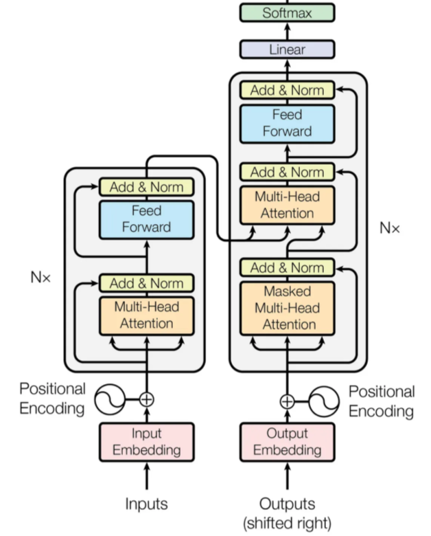
In the above figure, you can see the Input and Output embedding modules. During both training and inference, tokenization happens before the embedding process. Later, we will see that this embedding step is called Token Representation.
Part I: Tokenization
1.1 What Are Tokens and Tokenization?
Throughout this article, the word token is used frequently. A token is a discrete unit of information processed by a model. In the domain of language models, a token usually represents a word, part of a word, a punctuation mark, or another piece of text. In other domains, however, tokens may represent image patches, audio segments, time-series windows, and so on.
Before a model can process an input, it must first convert it into a sequence of tokens. The tokens themselves are not directly understood by the neural network. Instead, they must be converted into numbers using the model’s vocabulary, which is a fixed master list of every token the model is trained to recognize.
The total number of unique items in this list is the vocabulary size. Each token is mapped to its exact index number in this vocabulary, known as a Token ID. These token IDs are then transformed into meaningful vectors through an embedding layer (like those in the figure), producing numerical representations that the model can process.
As a result, the pipeline looks as follows:
The process of converting an input into tokens is called tokenization. Let’s look at an example of the first two steps of the above process:
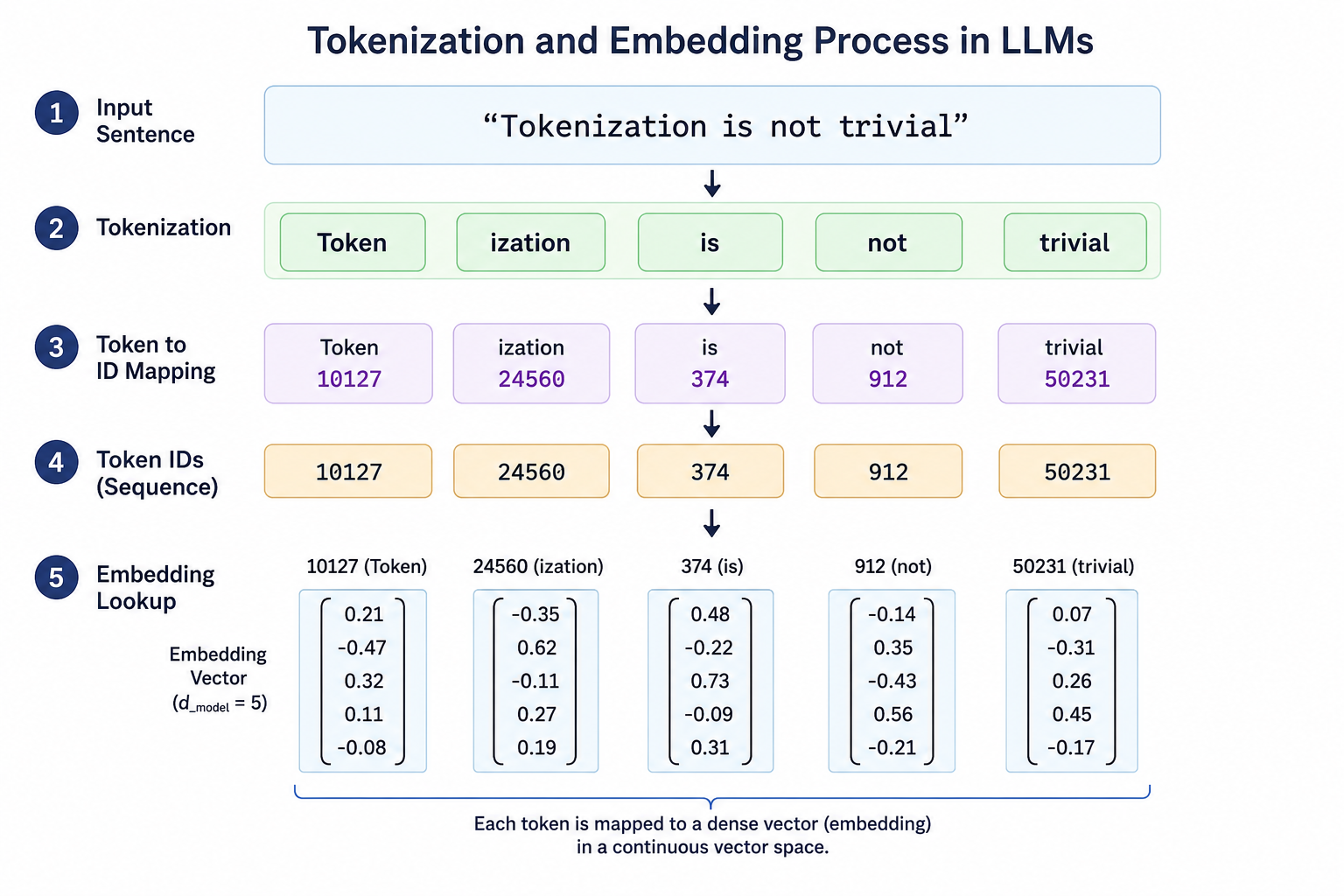
Example:
Let’s see how a simple sentence moves through the first two steps of the pipeline using a standard subword tokenizer (like the one used by GPT models).
-
Input (Raw Text):
"Tokenization is not trivial" -
Tokens (Discrete Units): The tokenizer chops the text into pieces. Notice how “Tokenization” is broken into smaller subword units: [
Token,ization,is,not,trivial] -
Token IDs (Unique Integers): Each token is looked up in the model’s pre-defined vocabulary dictionary and replaced by its corresponding mathematical ID: $[10127, 24560, 374, 912, 50231]$
Why do we need Token IDs after Tokenization?
It is tempting to think that once we split a sentence into string-based tokens like ["Token", "ization", "is", "not", "trivial"], the hard part is over. However, computers and neural networks cannot perform mathematical operations on raw text strings. They operate strictly on matrices and vectors of floating-point numbers.
Token IDs act as the bridge. By assigning every unique token in our vocabulary a fixed, unique integer index (e.g., Token $\rightarrow$ 10127), we create a structured lookup system that the neural network can interact with mathematically.
Think of this lookup table as a simple, two-way dictionary that handles two distinct phases:
-
Token to ID (Encoding): When processing your input text, the system looks up each string token to find its corresponding index number. \(\text{`Token`} \longrightarrow \text{Lookup Table} \longrightarrow 10127\)
-
ID to Token (Decoding): When the model generates a response, it outputs a raw number. This number is run backward through the exact same table to turn it back into a readable word for humans. \(10127 \longrightarrow \text{Lookup Table} \longrightarrow \text{`Token`}\)
Where Do These Numbers Come From?
A natural question arises: how do we come up with these specific numbers in the first place?
This mapping is neither random nor done manually. The process of tokenization is handled via a Tokenizer Model (such as Byte-Pair Encoding or WordPiece). Before the main Large Language Model (LLM) can even begin reading text, this tokenizer model must go through its own independent training phase.
When we say a tokenizer is “trained,” we do not mean it uses complex neural networks. Instead, tokenizer training is a statistical optimization process. Its entire goal is to read a massive sample dataset of raw text, analyze it, and find the most efficient balance between character-level chunks and whole-word chunks to build its vocabulary list.
1.2 Tokenization Methods
Modern LLMs rely on three primary algorithmic flavors to construct their vocabulary:
-
Byte-Pair Encoding (BPE): Starts with individual characters and iteratively merges the most frequent adjacent pairs. (Used by: GPT models, LLaMA).
-
WordPiece: Similar to BPE, but instead of choosing the most frequent pair, it picks pairs based on a statistical likelihood that maximizes predictability. (Used by: BERT).
-
Unigram: Starts with a massive vocabulary of full words and iteratively removes (prunes) the least useful tokens. (Used by: T5).
In the following sections, we describe these three methods individually.
1.2.1 Byte-Pair Encoding (BPE)
Byte-Pair Encoding (BPE) is a bottom-up subword tokenization method. It starts from a small base alphabet, usually characters or bytes, and gradually builds larger units by merging frequent adjacent pairs.
BPE was not originally designed for language models. It comes from data compression: the idea was to replace frequently repeated symbol pairs with a new symbol, making the sequence shorter. Modern NLP adapted the same idea for tokenization. Instead of only compressing text, BPE also produces a vocabulary of useful subword units.
Intuition
The core idea is:
\[\text{frequent pair} \quad \Rightarrow \quad \text{good candidate for a new token}\]For example, if the pair d + e appears many times in the corpus, BPE may create a new token de. Later, if de + r is frequent, it may create der. In this way, BPE gradually builds larger subwords and sometimes full words.
How BPE is Trained
-
Start from a base vocabulary The corpus is first represented using a small set of atomic symbols, such as characters or bytes. In some versions, an end-of-word marker like
</s>is added so that the algorithm can distinguish word boundaries. -
Count adjacent pairs BPE scans the corpus and counts how often each neighboring pair of symbols appears. For example, it may count pairs such as
de,er,th, orin. -
Choose the best immediate merge The most frequent adjacent pair is selected. This is a greedy decision: BPE chooses the merge that gives the largest immediate reduction in sequence length.
If a pair appears many times, replacing each occurrence of two symbols by one new symbol shortens the corpus:
\[(a, b) \rightarrow ab\] -
Update the corpus All selected occurrences of that pair are replaced by the new merged token. The corpus is now represented using this larger unit.
-
Repeat until the vocabulary budget is reached The algorithm repeats this process until it has learned the desired number of merge rules or reached the target vocabulary size.
A Mathematical Perspective
From a mathematical perspective, BPE is trying to find a sequence of merges:
\[\mu = (\mu_1, \mu_2, \dots, \mu_M)\]that maximizes the compression utility of the corpus:
\[\kappa_x(\mu)\]Here, $\kappa_x(\mu)$ measures how much shorter the sequence becomes after applying the merge sequence $\mu$. The ideal objective would be:
\[\mu^\star = \arg\max_{\mu} \kappa_x(\mu)\]However, standard BPE does not search over all possible merge sequences, as that would be computationally expensive. Instead, it uses a greedy approximation: at each step, it chooses the merge with the best immediate gain.
Algorithm 3 of the paper A Formal Perspective on Byte-Pair Encoding gives a useful way to understand what “optimal BPE” would mean.
-
Standard BPE is greedy: at each step, it merges the most frequent adjacent pair. This gives the best immediate compression gain, but it does not guarantee the best final vocabulary. A merge that looks good now may prevent a better sequence of merges later.
-
Algorithm 3 takes a different approach. Instead of committing immediately to the most frequent pair, it searches over possible merge sequences and keeps the sequence that gives the best final compression. In other words, standard BPE asks, “Which pair should I merge now?”, while Algorithm 3 asks, “Which full sequence of merges gives the shortest final representation?”
This makes Algorithm 3 an exact method for finding an optimal BPE vocabulary under the compression objective. However, it is computationally expensive, so it is mainly useful for theoretical analysis rather than for training large real-world tokenizers.
For a practical and minimal implementation of standard BPE, Andrej Karpathy’s minbpe repository is a good reference. It implements the usual greedy version of BPE: count adjacent pairs, merge the most frequent pair, update the text, and repeat. This is different from Algorithm 3 in the formal paper, which searches for an optimal merge sequence. So minbpe is useful for understanding how BPE is used in practice, while Algorithm 3 is useful for understanding what an optimal BPE vocabulary would mean mathematically.
1.2.2 WordPiece
WordPiece is another bottom-up subword tokenization method, heavily utilized by models like BERT and DistilBERT. Structurally, it is similar to BPE: both start from a base alphabet and iteratively expand the vocabulary. However, its merging strategy is grounded in probability and information theory rather than raw frequency.
Intuition
A pair is a good merge candidate not because it is common, but because it is more common together than its individual frequencies would predict.
How WordPiece is Trained
-
Initialize the vocabulary
Start with every individual character, punctuation mark, and special symbol found in the corpus (e.g.,
p,h,e,t,##e,##t…). The##prefix marks a character as one that only ever appears inside a word, never at its start — this is what lets the tokenizer later distinguish##ing(a suffix) froming(a standalone word). -
Count pair frequencies
Scan the corpus and count how often each adjacent symbol pair occurs — both together, e.g.
Count(p, ##h), and individually, e.g.Count(p)andCount(##h). -
Score all adjacent pairs
For every neighboring pair $(a, b)$, compute:
\[\text{Score}(a, b) = \frac{\text{Count}(ab)}{\text{Count}(a) \text{Count}(b)}\]This score is high when $a$ and $b$ co-occur more often than their individual frequencies would predict — not simply when $ab$ is common.
-
Merge the highest-scoring pair
The pair with the highest score is merged into a new token. For instance, if
##pand##hscore highest, they merge into##ph, which is added to the vocabulary. -
Repeat until the vocabulary budget is reached
Re-scan the (now updated) corpus with the new token in place, recompute scores, and merge again. This repeats — one merge per iteration — until the vocabulary reaches its target size (e.g., 30,000 tokens).
The scoring formula introduced above,
\[\text{score}(a,b) = \frac{\text{Count}(a,b)}{\text{Count}(a)\,\text{Count}(b)}\]is often described as Pointwise Mutual Information or PMI. It is close, but not exact.
For two discrete events $x$ and $y$, PMI is defined as:
\[\operatorname{PMI}(x,y)=\log \frac{p(x,y)}{p(x)p(y)}\]where
- $p(x,y)$ is the joint probability of observing $x$ and $y$ together,
- $p(x)$ is the marginal probability of observing $x$,
- $p(y)$ is the marginal probability of observing $y$.
Equivalently, PMI can be written as:
\[\operatorname{PMI}(x,y)=\log \frac{p(x \mid y)}{p(x)}=\log \frac{p(y \mid x)}{p(y)}\]A Mathematical Perspective
In the WordPiece score equation, if we write each count as a probability by dividing by the total number of tokens $N$: \(P(a) = \text{Count}(a)/N\), then
\[\frac{P(a,b)}{P(a)P(b)} = \frac{\text{Count}(a,b)/N}{\big(\text{Count}(a)/N\big)\big(\text{Count}(b)/N\big)} = N \cdot \frac{\text{Count}(a,b)}{\text{Count}(a)\,\text{Count}(b)} = N \cdot \text{score}(a,b)\]Therefore,
\[\log \frac{P(a,b)}{P(a)P(b)} = \log\big(N \cdot \text{score}(a,b)\big) = \log N + \log\,\text{score}(a,b)\]At any single training step, this constant $N$ is the same for every candidate pair. Therefore, ranking pairs by $\text{score}(a,b)$ is equivalent to ranking them by the PMI-like quantity above. However, there are two important differences: Asymmetry and The Dynamic Probability Space.
Asymmetry
Classical PMI is symmetric, $\text{PMI}(x;y) = \text{PMI}(y;x)$, but the WordPiece score is not, because $ab$ is different from $ba$. In probability language, $\text{PMI}(a,b)$ measures the association between $a$ and $b$ in the whole corpus, regardless of their order. On the other hand, $\text{score}(a,b)$ measures co-occurrence of $a$ and $b$ in this exact order, where $b$ appears immediately after $a$. So
\[\text{Count}(a,b) \neq \text{Count}(b,a)\]The algorithm is scoring directed sequential adjacency, not undirected association.
The Dynamic Probability Space
The training algorithm never optimizes against a fixed distribution. After each merge, the corpus representation changes and becomes shorter. Every merge changes the counts that the next merge’s scores depend on. When $a$ and $b$ merge into $ab$, three things shift in the corpus simultaneously:
- $\text{Count}(a)$ and $\text{Count}(b)$ both decrease (every merged occurrence is no longer counted as a standalone $a$ or $b$).
- $\text{Count}(ab)$ appears for the first time.
- Every other pair in the corpus that contains $a$ or $b$ has its own score affected, since its denominator terms just changed.
Because the landscape shifts after every merge, WordPiece is a greedy algorithm in a genuine, consequential sense. However, in the classical PMI definition, the distribution is fixed.
Mathematical Bounds: Maximums and Minimums
Using the simpler ratio-only score:
- Minimum ($0$): the score is exactly $0$ when $A$ and $B$ never appear adjacent, $\text{Count}(a,b) = 0$. Pairs with large individual frequencies but negligible co-occurrence approach $0$ as well.
- Maximum ($1$): since $\text{Count}(a,b)$ can never exceed $\text{Count}(a)$ or $\text{Count}(b)$, $1$ is the theoretical ceiling. It is reached only when $A$ and $B$ perfectly co-occur — they only ever appear together, so $\text{Count}(a,b) = \text{Count}(a) = \text{Count}(b) = k$, giving $\text{score}(a,b) = k/(k \times k) = 1/k$. Hitting the true maximum of $1$ requires $k = 1$: the highest possible score belongs to a pair that occurs adjacent exactly once in the entire corpus and nowhere else.
Standard WordPiece vs. Fast WordPiece
When exploring WordPiece implementations, a distinction is frequently made between Standard WordPiece and Fast WordPiece (often associated with Google’s linear-time implementations and Hugging Face’s Rust-based tokenizers library). This distinction centers purely on the execution efficiency of the tokenization step rather than the underlying vocabulary rules.
Standard WordPiece
Suppose we are given a word with $m$ characters and vocabulary size of $n$.
One way to describe the cost is in terms of vocabulary lookup. If each candidate substring must be compared naively against a vocabulary of size $n$, then in the worst case the tokenizer may perform as many as $[\mathcal{O}(mn)]$ comparisons: for each of the $m$ possible character positions, it may need to search through all vocabulary entries to find whether a valid token exists.
Therefore, the inefficiency of standard WordPiece does not come from the vocabulary itself. It comes from the search procedure.
This is why standard WordPiece is often described as having worst-case complexity around $[\mathcal{O}(m^2)]$ or, depending on the lookup implementation, $[\mathcal{O}(mn)]$. For large-scale pretraining, where billions or trillions of words must be tokenized, this repeated backtracking can become a significant bottleneck.
- Note: In practice, vocabularies are usually stored in hash tables or tries, so lookup is much faster than a naive scan over all $n$ tokens.
Fast WordPiece
Fast WordPiece eliminates backtracking entirely by modeling the vocabulary as a specialized data structure known as a Trie (a prefix tree), augmented with advanced search mechanisms inspired by the Aho-Corasick string-matching algorithm.
- Failure Links & Failure Pops: In Fast WordPiece, every node in the vocabulary trie contains precomputed “failure links”. If the tokenizer is stepping through the tree matching characters (e.g., tracking
s$\rightarrow$t$\rightarrow$r$\rightarrow$a) and hits a character that fails to match an edge, it does not reset and backtrack to the beginning of the word. Instead, it immediately follows a failure link to another precomputed node in the trie where a valid sub-match exists, emitting the tokens along the way (“failure pops”). - Single-Pass End-to-End Processing: While standard tokenizers use a two-step approach—first splitting an entire sentence into raw words using whitespace and punctuation (pre-tokenization) and then passing each word individually to the subword loop—Fast WordPiece handles both simultaneously. It streams the entire raw sentence text through the trie in a single linear pass.
As a result, Fast WordPiece processes text in strict $\mathcal{O}(n)$ time complexity relative to the sentence length $n$, executing up to 5 to 8 times faster than traditional implementations without altering the final tokenized output.
1.2.3 BPE and WordPiece Comparison
Concrete Tokenization Examples
To illustrate how these trained vocabularies behave in practice, let us examine how BPE and WordPiece process a sample sentence once training is complete.
Assume both tokenizers have been trained on an English corpus containing a mix of common and rare words, resulting in the following simplified vocabularies:
- BPE Vocabulary:
["the", "cat", "walk", "ed", "strang", "ely", "s", "a", "b", "c", ...](plus the end-of-word marker</s>) - WordPiece Vocabulary:
["the", "cat", "walk", "##ed", "strang", "##ely", "##e", "a", "b", "c", ...]
BPE Tokenization Example
Input word: "strangely"
- The word is split into individual characters with an end-of-word marker:
s t r a n g e l y </s> - The tokenizer scans its merge rules list. The earliest rule matching any pair here is the one that created
strang. The sequence becomes:strang e l y </s> - The next highest-priority merge rule in the vocabulary is for
ely. The sequence becomes:strangely</s> - No further valid merge rules apply.
- Final BPE Tokens:
["strang", "ely</s>"](often rendered simply as["strang", "ely"]with space indicators likeĠstrang,elydepending on the exact implementation).
- Final BPE Tokens:
WordPiece Tokenization Example
WordPiece tokenizes text in a top-down, greedy fashion using an algorithm called MaxMatch (Maximum Matching). Instead of executing merge rules chronologically, it scans an isolated word from left to right, hunting for the longest string starting from the current position that exists in the vocabulary.
Input word: "strangely"
- It looks at the whole string
"strangely". It is not in the vocabulary. - It chops letters off the end until it finds a match:
"strangely"$\rightarrow$"strangel"$\rightarrow$"strange"$\rightarrow$"strang"(Match found!). - The remaining substring is
"ely". Because it is a continuation of a word, the tokenizer looks for pieces prefixed with##. - It looks for
"##ely". (Match found!).- Final WordPiece Tokens:
["strang", "##ely"]
- Final WordPiece Tokens:
The [UNK] Token
The role of [UNK] becomes clear if we ask a simple question:
What are the smallest units the tokenizer is allowed to use?
A tokenizer can only decompose text into units that exist in its vocabulary. If the smallest units are characters, then every character that may appear at inference time must already be known. If the tokenizer sees a character that was never included in its base vocabulary, it has no smaller unit to fall back to.
This is the situation with standard WordPiece.
Suppose the WordPiece vocabulary was built from English text and contains characters such as: a, b, c, …, z.
Now imagine the model receives the word: cat🙂
The tokenizer can handle c, a, and t, but if the emoji 🙂 was never included in the base vocabulary, WordPiece cannot split it any further. The emoji is already a single Unicode character from the tokenizer’s point of view. There is no smaller known unit available. Therefore, the tokenizer gives up and outputs: [UNK]
The same problem can happen with rare mathematical symbols, foreign alphabets, or unusual Unicode characters. The issue is not that WordPiece is “bad”; the issue is that its fallback level is usually the character level, and the vocabulary is not rich enough to cover every possible input.
Classical BPE can have the same problem if it also starts from a fixed character vocabulary.
Byte-level BPE solves this by moving the fallback level to bytes.
Instead of starting from characters, byte-level BPE starts from bytes. Every text string on a computer can be represented as a sequence of bytes, for example using UTF-8 encoding. Therefore, the base vocabulary has at least 256 possible byte values.
Byte-level BPE includes all 256 bytes in its base vocabulary. Therefore, even if the tokenizer sees a completely new character, it can always decompose that character into its underlying bytes.
For example, 🙂 may be unknown as a character, but it is still representable as a sequence of UTF-8 bytes. Since those bytes are guaranteed to exist in the vocabulary, the tokenizer never gets stuck.
This is why WordPiece usually needs an explicit [UNK] token, while byte-level BPE can avoid it.
1.2.4 Unigram
BPE and WordPiece are usually described as bottom-up tokenization algorithms. They start from small units, such as characters or bytes, and gradually build larger subword tokens.
The Unigram Language Model, usually just called Unigram, takes the opposite direction. It starts with a very large vocabulary of candidate pieces and then gradually removes the least useful ones. In that sense, Unigram is a top-down pruning algorithm — the mirror image of BPE and WordPiece, which are bottom-up and grow their vocabulary one merge at a time. Unigram is used in SentencePiece (section 1.3), especially in models such as T5.
This immediately raises two questions: where does that “very large” initial vocabulary come from, and once we have it, what criterion decides which pieces survive? The rest of this section answers both.
How Is the Initial Vocabulary Built?
Unigram starts with a large initial vocabulary. This vocabulary is intentionally bigger than the final target vocabulary.
In practice, the initial vocabulary usually contains:
- frequent full words from the corpus,
- frequent substrings,
- character-level units,
- special tokens such as
<unk>,<s>,</s>, or padding tokens, - whitespace-aware pieces such as
▁the,▁is, or▁Tokenin SentencePiece. The initial vocabulary must be large because Unigram is a pruning method. If a useful token is not present in the initial candidate set, the algorithm cannot recover it later. This is different from BPE, where new tokens are created by merging smaller units. Instead, it treats tokenization as a probabilistic segmentation problem.
In practice, this seed vocabulary is not built by hand — it is generated automatically from the corpus, and it has to be built in a way that stays computationally cheap even though it may contain hundreds of thousands of candidate substrings. The two common approaches are:
- Seed with BPE. Run a few thousand iterations of ordinary BPE and keep every intermediate merge ever produced (not just the final vocabulary) as a candidate piece.
- Seed with an Enhanced Suffix Array (ESA). This is the approach used by the original SentencePiece implementation. A suffix array lets you enumerate every repeated substring of the corpus, together with its frequency, in roughly linear time — instead of the quadratic cost of naively checking every substring against every other one. The ESA is then used to pull out the most frequent substrings up to some maximum length, which become the seed pieces.
Either way, the seed vocabulary is deliberately redundant: it contains overlapping candidates (
un,believ,able,believable,unbelievable, …) precisely so that the pruning step described below has real alternatives to choose between.
For example, consider the word unbelievable. Suppose the seed vocabulary contains all of the following pieces, so the word admits four different segmentations:
- [
un,believable] - [
un,believ,able] - [
unbelievable] - [
un,bel,iev,able] Unigram assigns a probability to every individual piece in the vocabulary, not to a segmentation directly —p(un),p(believable),p(believ),p(able), and so on. Once we have these per-piece probabilities, each of the four segmentations above gets its own probability, and the tokenizer prefers whichever segmentation scores highest. The next part of this section makes that precise: what exactly is being multiplied together, what the training objective (loss function) is, why that particular function qualifies as a loss, and how the pruning step actually decides which pieces to throw away.
A More Correct Mathematical View of Unigram
1. The generative model behind the name “Unigram”
Let $V$ be the current vocabulary, and let $p(x)$ denote the probability assigned to piece $x \in V$. These probabilities form a proper distribution over the vocabulary:
\[\sum_{x \in V} p(x) = 1, \qquad p(x) \geq 0 \; \; \forall x \in V\]Given an input string $X$ (a word, or a whitespace-escaped sentence — see section 1.3), a segmentation is a sequence $\mathbf{x} = (x_1, x_2, \dots, x_m)$ of pieces from $V$ whose concatenation reconstructs $X$. Let $S(X)$ denote the set of all valid segmentations of $X$ — for unbelievable, this is exactly the four candidates listed above.
The model gets its name from a specific, deliberately simple independence assumption: the probability of a segmentation is just the product of the probabilities of its pieces, with no dependence on neighboring pieces — the probability of able does not change depending on whether it follows believ or bel iev. This is the same “bag of independent draws” assumption behind classical unigram language models and Naive Bayes classifiers:
This is a strong simplification — a real language model would want $p(x_i \mid x_{i-1})$ or richer context — but it buys tractability: with no dependence between pieces, finding the best segmentation reduces to a shortest-path problem instead of an exponential search.
2. Picking a segmentation
Given the piece probabilities, the best tokenization of $X$ is the highest-probability segmentation:
\[\mathbf{x}^\star = \arg\max_{\mathbf{x} \in S(X)} P(\mathbf{x}) = \arg\max_{\mathbf{x} \in S(X)} \prod_{i=1}^m p(x_i)\]Taking logs does not change the arg max (log is monotonic), and it turns a product into a sum:
\[\mathbf{x}^\star = \arg\max_{\mathbf{x} \in S(X)} \sum_{i=1}^m \log p(x_i)\]This is now a search for the highest-weight path through a small directed acyclic graph.
3. The loss function: negative log-likelihood of the corpus
Training means choosing the probabilities $p(x)$ that best explain a training corpus $D = {X_1, \dots, X_N}$. The subtlety is this: the training objective does not use only the single best segmentation $\mathbf{x}^\star$. It uses the marginal probability of the sentence — the sum over every valid segmentation:
\[P(X) = \sum_{\mathbf{x} \in S(X)} P(\mathbf{x}) = \sum_{\mathbf{x} \in S(X)} \prod_{i=1}^m p(x_i)\]Summing over the hidden segmentation, rather than only keeping the best one, matters: a piece can be genuinely useful even when it never wins the argmax, simply by contributing to many near-optimal segmentations. The loss function for the whole corpus is the negative log-likelihood:
\[\mathcal{L}(p) = -\sum_{s=1}^{N} \log P(X_s) = -\sum_{s=1}^{N} \log \left( \sum_{\mathbf{x} \in S(X_s)} \prod_{i=1}^{m_s} p(x_i) \right)\]Training the Unigram model means solving:
\[p^\star = \arg\min_{p} \; \mathcal{L}(p) \quad \text{subject to} \quad \sum_{x \in V} p(x) = 1\]4. Training loop: Expectation-Maximization plus pruning
Putting the pieces together, one full Unigram training run looks like this:
- Build a large seed vocabulary $V_0$ using BPE or ESA-based substring statistics, as described above.
- Initialize $p(x)$ for every $x \in V_0$, e.g., from relative frequency of that substring in the seed statistics, normalized so probabilities sum to 1.
- E-step. For each sentence in the corpus, run the forward-backward algorithm (Viterbi’s “soft” cousin) over $S(X_s)$ to compute the expected count of every piece — i.e., how often piece $x$ is used, averaged over all segmentations weighted by their probability under the current $p$, not just the single best one.
- M-step. Re-estimate each $p(x)$ as its expected count divided by the total expected count across the vocabulary — the closed-form MLE update given the expectations from step 3. This is a standard EM iteration; it is guaranteed not to increase $\mathcal{L}(p)$.
- Score each piece by its removal cost. For every $x \in V$, compute how much the total corpus loss $\mathcal{L}(p)$ would increase if $x$ were deleted from the vocabulary and every sentence that used it had to fall back to its next-best segmentation. Pieces with the smallest loss-increase are the ones the model can most easily do without.
- Prune. Remove the bottom fraction (commonly the worst 10–20%) of pieces by this score. Single characters are typically protected from pruning, so the vocabulary can never become unable to represent some input (avoiding the
[UNK]problem discussed in section 1.2.2). -
Repeat steps 3–6 until $ V $ reaches the target vocabulary size.
5. A numeric walk-through, continuing the unbelievable example
Suppose, at some point during training, the model has learned these (illustrative, not real) piece probabilities:
| Piece | $p(x)$ |
|---|---|
un |
0.020 |
believable |
0.00030 |
believ |
0.0010 |
able |
0.010 |
unbelievable |
0.00005 |
bel |
0.020 |
iev |
0.00070 |
Each of the four segmentations gets a probability under the independence assumption $P(\mathbf{x}) = \prod_i p(x_i)$:
\[\begin{aligned} P_1 &= p(\texttt{un}) \cdot p(\texttt{believable}) &&= 0.020 \times 0.00030 &&= 6.0 \times 10^{-6} \\ P_2 &= p(\texttt{un}) \cdot p(\texttt{believ}) \cdot p(\texttt{able}) &&= 0.020 \times 0.0010 \times 0.010 &&= 2.0 \times 10^{-7} \\ P_3 &= p(\texttt{unbelievable}) &&&&= 5.0 \times 10^{-5} \\ P_4 &= p(\texttt{un}) \cdot p(\texttt{bel}) \cdot p(\texttt{iev}) \cdot p(\texttt{able}) &&= 0.020 \times 0.020 \times 0.00070 \times 0.010 &&= 2.8 \times 10^{-9} \end{aligned}\]Best segmentation (Viterbi): $P_3$ is the largest single term, so $\mathbf{x}^\star = [\texttt{unbelievable}]$ — the tokenizer keeps the word whole.
Marginal probability (used in the loss): sum over all four,
\[P(X) = P_1 + P_2 + P_3 + P_4 \approx 6.0\times10^{-6} + 2.0\times10^{-7} + 5.0\times10^{-5} + 2.8\times10^{-9} \approx 5.62 \times 10^{-5}\]so this word’s contribution to $\mathcal{L}(p)$ is $-\log(5.62\times10^{-5}) \approx 9.79$.
What pruning unbelievable would cost: if the piece unbelievable were removed from the vocabulary, $P_3$ disappears and only three segmentations remain:
This gives a new loss contribution of $-\log(6.2\times10^{-6})$, which is larger than before. Therefore, removing unbelievable increases the loss for this word. Summed over every word in the corpus that used this piece, that total increase is exactly the “removal cost” from step 5 above. If some other candidate piece’s total removal cost across the whole corpus were smaller than this, it would be pruned first.
1.2.5 Bringing It All Together: BPE vs. WordPiece vs. Unigram
With all three algorithms on the table, it is useful to compare them directly along the axes that actually distinguish them:
| BPE | WordPiece | Unigram | |
|---|---|---|---|
| Direction | Bottom-up (grows the vocabulary) | Bottom-up (grows the vocabulary) | Top-down (shrinks the vocabulary) |
| Starting point | Base characters/bytes | Base characters/bytes | A large seed vocabulary (from BPE or ESA substring statistics) |
| Selection criterion | Raw pair frequency | PMI-like co-occurrence score, $\text{Count}(ab)/(\text{Count}(a)\text{Count}(b))$ | Global corpus negative log-likelihood, $\mathcal{L}(p)$, optimized via EM |
| What each step does | Merges the most frequent adjacent pair | Merges the pair with the highest likelihood-ratio score | Removes the piece(s) with the smallest loss-increase upon removal |
| Is the objective probabilistic? | No — purely frequency-driven | Partially — score is likelihood-flavored, but not a normalized probability model | Yes — pieces have a proper probability distribution $p(x)$ over the whole vocabulary |
| Tokenization at inference | Deterministic: apply learned merge rules in order | Deterministic: greedy longest-match (MaxMatch) | Naturally probabilistic: Viterbi picks the single best segmentation, but the model can also sample alternative segmentations |
| Handles segmentation ambiguity? | No — one fixed set of merge rules, one output | No — one fixed greedy scan, one output | Yes, explicitly — the loss itself sums over every valid segmentation, and training can even use “subword regularization” (sampling non-optimal segmentations) to make downstream models robust to tokenization noise |
| Typical users | GPT, LLaMA (usually byte-level) | BERT, DistilBERT | T5 and other SentencePiece-based models |
The direction each algorithm moves in is really a consequence of what it is optimizing. BPE only ever asks a local question — “which adjacent pair is most frequent, right now?” — so it has no way to remove a bad early decision later; it can only build on top of it. Unigram instead evaluates candidates against one global objective, $\mathcal{L}(p)$, computed over the entire corpus, which is exactly what makes pruning coherent: a piece is judged by how much the whole vocabulary’s fit degrades without it, not by a local pairwise statistic. That global, probabilistic view is also what buys Unigram its two extra abilities that BPE and WordPiece do not have: a principled notion of “how good is this vocabulary” ($\mathcal{L}(p)$ itself), and the ability to represent genuine tokenization ambiguity instead of collapsing every input to one fixed output.
1.3 SentencePiece: The Language-Independent Framework
While BPE and WordPiece are powerful subword algorithms, they historically relied on a crucial first step: pre-tokenization. Before the algorithm could process the text, a script had to split the sentence into words based on spaces and punctuation (e.g., separating "I love AI." into ["I", "love", "AI", "."]).
This creates a serious problem for language models intended to be multilingual. Languages like Chinese, Japanese, and Thai do not use spaces to separate words. Furthermore, different languages have complex and varying rules for punctuation, hyphens, and apostrophes. Relying on spaces and hardcoded punctuation rules makes a tokenizer fundamentally language-dependent.
The SentencePiece Solution
SentencePiece, developed by Google, solves this by acting as a language-independent wrapper around algorithms like BPE or Unigram. It achieves this by skipping the pre-tokenization (word-splitting) step entirely.
Instead of discarding spaces, SentencePiece treats the entire input as a raw stream of characters and treats the space as just another standard letter.
- Whitespace Escaping: Before any subword algorithm is applied, SentencePiece replaces all spaces in the raw text with a special meta-symbol, usually the lower one-eighth block:
▁(U+2581).- Raw Text:
"Tokenization is not trivial" - Escaped:
"▁Tokenization▁is▁not▁trivial"
- Raw Text:
- Applying the Algorithm: This escaped string is then fed into the core subword algorithm (like BPE for LLaMA, or Unigram for T5). The algorithm splits the text into tokens, but the
▁remains physically attached to the beginning of the words.- Tokens:
["▁Token", "ization", "▁is", "▁not", "▁trivial"]
- Tokens:
Notice how "ization" does not have the ▁ marker. This is how the model structurally understands that "Token" and "ization" belong to the exact same word and should not have a space between them.
Lossless Detokenization
The most significant advantage of this approach becomes apparent during text generation (inference).
In older tokenizers, when the model generated a sequence of tokens, the system had to use hardcoded rules to figure out whether to put spaces between them (e.g., “Add a space between words, but do not add a space before a period or a comma”).
With SentencePiece, the detokenization process is mathematically lossless and rule-free. It requires zero language-specific rules. The pipeline simply reverses the escaping process:
- Concatenation: The generated string tokens are glued together exactly as they are output by the model.
(
"▁Token" + "ization" + "▁is" + "▁not" + "▁trivial"$\rightarrow$"▁Tokenization▁is▁not▁trivial!") - Replacement: The system performs a basic find-and-replace, swapping every
▁symbol back into a standard, invisible whitespace. (" Tokenization is not trivial!")
Because SentencePiece is an overarching framework, it is highly versatile. When you load a modern model like T5 or LLaMA, Hugging Face quietly uses the SentencePiece library in the background to handle this precise ▁ spacing logic before passing the mathematical Token IDs to the model.
1.4 How Do We Evaluate a Tokenizer?
Because tokenizers determine how efficiently a model processes text, it is important to measure their performance. Researchers look at a few key areas:
- Compression Rate: This measures how many tokens are needed to represent a single word on average. A lower score is better because it means the tokenizer is efficient. If one tokenizer needs 5 tokens to read the word “unbelievable” and another needs only 2, the second one uses the model’s capacity much better.
- Unknown Word Rate: How often does the tokenizer have to use the
[UNK](Unknown) token? Modern tokenizers that can fall back to basic bytes usually have a rate of 0%, which is the ideal goal. - Fairness Across Languages: Models that handle multiple languages are tested on how equally they treat them. If a tokenizer needs 1 token for an English sentence but 4 tokens for a sentence with the same meaning in Turkish, the model will be slower and more expensive to run for Turkish users. A good tokenizer works efficiently across many different languages.
1.5 Some Remarks on Tokenization
1- The Golden Rule: Once Learned, It is Frozen
Once the tokenizer algorithm finishes its training phase and locks in its vocabulary table, the ID for a specific token is fixed. For example, the token "pug" will always map to the integer ID 4. Whether the model is being trained to understand language or is generating text for a user, this lookup table remains completely frozen. In short: Token IDs are entirely fixed and never change during LLM inference.
2- The Multi-Step Role of the Tokenizer
While we often use “tokenization” to refer to the whole text-to-ID pipeline, the tokenizer object in modern NLP libraries (like Hugging Face) actually handles several distinct steps in sequence:
- Normalization: Cleaning the text (e.g., stripping whitespace, handling casing, removing accents).
- Pre-tokenization: Splitting the raw text into rough boundaries, usually by spaces or punctuation.
- Model Tokenization: Applying a core algorithmic rule (like BPE) to split words into subwords.
- Post-Processing: Injecting model-specific special tokens (such as
[CLS],[SEP], or<|endoftext|>). - ID Mapping: Converting the final array of tokens into their corresponding Token IDs.
Part II: Token Representation
2.1 From Integers to Meaning
At the end of the tokenization pipeline, we are left with an array of Token IDs — a sequence of integers like [30121, 1634, 318, 1257, 0]. While computers can process numbers, these raw integers are fundamentally inadequate for a neural network to understand language.
This matters because Token IDs are categorical, not quantitative.
If the token "king" is assigned ID 1000 and the token "apple" is assigned ID 1001, the mathematical proximity of these two numbers means absolutely nothing. They are just arbitrary labels. A neural network cannot multiply or add these IDs together to extract grammar, context, or meaning.
This is where Token Representation (commonly referred to as Embedding) comes in. Token representation is the process of translating these rigid, arbitrary integers into rich, continuous mathematical objects called vectors.
2.2 The Embedding Layer: Building the Vector
Before the discrete Token IDs enter the deep layers of the Transformer (like the Attention mechanisms), they pass through the Embedding Layer. You can think of this layer as a massive lookup table, but instead of mapping a string to an integer, it maps an integer to a high-dimensional list of floating-point numbers.
Instead of representing "Token" as a single number (30121), the embedding layer represents it as a dense vector of hundreds or thousands of dimensions (often denoted as $d_{\text{model}}$):
Each dimension in this vector captures a tiny, abstract fraction of the token’s semantic meaning. In this high-dimensional space, words with similar meanings (like "king" and "queen") end up mathematically closer together, while unrelated words (like "king" and "toaster") are pushed far apart.
2.3 The Core Differences: Tokenization vs. Representation
To build a clear mental map, it is crucial to separate these two phases conceptually. Here is how tokenization and token representation differ:
- Fixed vs. Learned:
- Tokenization is a fixed, pre-processing step. Once the tokenizer is trained and its vocabulary dictionary is locked in, the ID for a specific token never changes. The word
"the"will always be1996in a BERT model. - Token Representation is a dynamic, learned process. The vector assigned to ID
1996starts as random noise and is continuously updated and refined via backpropagation during the LLM’s training phase. The model learns what the token means by adjusting these floating-point numbers.
- Tokenization is a fixed, pre-processing step. Once the tokenizer is trained and its vocabulary dictionary is locked in, the ID for a specific token never changes. The word
- Syntax vs. Semantics:
- Tokenization only cares about syntax and structure. It is a statistical machine that asks: “How do I efficiently chop this string of characters into smaller pieces?” It has no understanding of what the words actually mean.
- Token Representation cares entirely about semantics. It asks: “What is the underlying meaning of this discrete piece, and how does it relate to all the other pieces in my vocabulary?”
- Hardware Execution:
- Tokenization is almost always executed on the CPU. It is a software-level string manipulation task using dictionaries, tries, or regular expressions.
- Token Representation happens on the GPU (or TPU). The embedding layer is the very first true layer of the neural network, performing massive matrix multiplications.
In summary, if tokenization is the act of giving every word a unique ID badge to enter the building, token representation is the process of reading that badge to understand the person’s entire background, skills, and relationship to everyone else in the room.
2.4 Why We Cannot Simply Change the Tokenizer
When working with pre-trained models, developers often ask: “Can I just add new words to the tokenizer or replace it with a better one?”
The short answer is: if you change the tokenizer, you break the embeddings.
Remember that the Embedding Layer is like a large lookup table. Each Token ID corresponds to a specific row in that table, which holds the vector (the mathematical meaning) for that token.
If you train the tokenizer again or change it, the IDs will get mixed up. For example, the word "apple" might move from ID 500 to ID 2104. If you give ID 2104 to the original model, it will look up row 2104, which used to belong to a completely different word. The result will be meaningless output.
How do we add new words, then? If you need to add new tokens (for example, for specific medical terms or a new language), you must carefully expand the model:
- Add the new tokens to the tokenizer’s vocabulary.
- Add new, empty rows to the bottom of the model’s embedding matrix so it gets larger.
- Fill these new rows with starting values. You can use random numbers, or you can average the values of the smaller pieces that used to make up the new word.
- Train the model again (fine-tune). You must train the model so it can learn the correct mathematical meaning for these newly added vectors.
Part III: Some Concrete Examples
3.1 Different Models, Different Tokenization
In the following example, I demonstrate how different models tokenize the same text. You can see the pipeline here: code. Everything (downloading and loading) is handled by the AutoTokenizer module in transformers library.
Text: Tokenization is not trivial.
| Model | Tokens | Token IDs |
|---|---|---|
| BERT WordPiece | [[CLS], token, ##ization, is, not, trivial, ., [SEP]] |
[101, 19204, 3989, 2003, 2025, 20610, 1012, 102] |
| GPT-2 Byte-level BPE | [Token, ization, Ġis, Ġnot, Ġtrivial, .] |
[30642, 1634, 318, 407, 20861, 13] |
| RoBERTa Byte-level BPE | [<s>, Token, ization, Ġis, Ġnot, Ġtrivial, ., </s>] |
[0, 45643, 1938, 16, 45, 30063, 4, 2] |
| T5 SentencePiece | [▁To, ken, ization, ▁is, ▁not, ▁trivia, l, ., </s>] |
[304, 2217, 1707, 19, 59, 22377, 40, 5, 1] |
| LLaMA-style tokenizer | [<s>, ▁Token, ization, ▁is, ▁not, ▁trivial, .] |
[1, 25159, 2133, 338, 451, 12604, 29889] |
| Qwen-small | [Token, ization, Ġis, Ġnot, Ġtrivial, .] |
[3323, 2022, 374, 537, 35647, 13] |
Text: unbelievable
| Model | Tokens | Token IDs |
|---|---|---|
| BERT WordPiece | [[CLS], unbelievable, [SEP]] |
[101, 23653, 102] |
| GPT-2 Byte-level BPE | [un, bel, iev, able] |
[403, 6667, 11203, 540] |
| RoBERTa Byte-level BPE | [<s>, un, bel, iev, able, </s>] |
[0, 879, 8494, 18421, 868, 2] |
| T5 SentencePiece | [▁unbelievable, </s>] |
[25525, 1] |
| LLaMA-style tokenizer | [<s>, ▁un, bel, iev, able] |
[1, 443, 6596, 10384, 519] |
| Qwen-small | [un, belie, vable] |
[359, 31798, 23760] |
Text: I love machine learning 😊
| Model | Tokens | Token IDs |
|---|---|---|
| BERT WordPiece | [[CLS], i, love, machine, learning, [UNK], [SEP]] |
[101, 1045, 2293, 3698, 4083, 100, 102] |
| GPT-2 Byte-level BPE | [I, Ġlove, Ġmachine, Ġlearning, ĠðŁĺ, Ĭ] |
[40, 1842, 4572, 4673, 30325, 232] |
| RoBERTa Byte-level BPE | [<s>, I, Ġlove, Ġmachine, Ġlearning, ĠðŁĺ, Ĭ, </s>] |
[0, 100, 657, 3563, 2239, 17841, 27969, 2] |
| T5 SentencePiece | [▁I, ▁love, ▁machine, ▁learning, ▁, <unk>, </s>] |
[27, 333, 1437, 1036, 3, 2, 1] |
| LLaMA-style tokenizer | [<s>, ▁I, ▁love, ▁machine, ▁learning, ▁, <0xF0>, <0x9F>, <0x98>, <0x8A>] |
[1, 306, 5360, 4933, 6509, 29871, 243, 162, 155, 141] |
| Qwen-small | [I, Ġlove, Ġmachine, Ġlearning, ĠðŁĺ, Ĭ] |
[40, 2948, 5662, 6832, 26525, 232] |
Key Takeaways from the Tables
Looking at how different models handle the exact same text shows us a few important differences:
- Handling Spaces: Notice how the models show spaces between words. GPT-2, RoBERTa, and Qwen use
Ġto represent a space. T5 and LLaMA use▁. BERT, however, removes spaces completely and uses##to show that a piece belongs to the preceding word (like##ization). - The Emoji Problem: Look at the example with the “😊” emoji. BERT does not recognize it and replaces it with an unknown token,
[UNK]. T5 also outputs<unk>. But GPT-2, RoBERTa, and LLaMA handle it smoothly by breaking the emoji down into basic computer bytes. LLaMA splits the emoji into its raw byte codes (like<0xF0>). This ensures the model does not lose the information, even if the exact emoji is not in its main vocabulary. - Different Word Splits: For the word “unbelievable”, every model makes a different choice. GPT-2 splits it into four parts (
un,bel,iev,able), while T5 keeps it as one complete word (▁unbelievable). This shows how a model’s training data and tokenizer design affect how it breaks down text.
3.2 What Are These Tokenizer Files on Hugging Face?
When you download a tokenizer from Hugging Face, you usually get several files rather than a single one. Together, they describe how text is split into tokens, how tokens are mapped to IDs, and how the model should use that tokenizer.
Common files include:
config.json
tokenizer.json
tokenizer_config.json
vocab.json
merges.txt
Not every tokenizer has all of them. The exact files depend on the tokenizer family (BPE, WordPiece, SentencePiece, etc.).
tokenizer.json
This is often the main tokenizer file. It usually stores the full tokenizer pipeline: normalization, pre-tokenization, subword model, post-processing, and decoding. In many Hugging Face fast tokenizers, this file is enough to reconstruct the tokenizer.
tokenizer_config.json
This contains Hugging Face-specific tokenizer settings, such as the tokenizer class, maximum input length, lowercasing behavior, padding/truncation defaults, and special token settings. It is more like wrapper metadata than the tokenizer algorithm itself.
vocab.json
This is the vocabulary dictionary: it maps token strings to integer token IDs. For example, it may store entries like
\[\texttt{"hello"} \to 31373\]It tells us which tokens exist and what IDs they have.
merges.txt
This appears in BPE tokenizers. It stores the ordered list of merge rules learned during BPE training. In other words, it helps define how smaller units are merged into larger subword tokens. That is why BPE tokenizers often need both vocab.json and merges.txt.
config.json
This one is usually the model configuration file, not the tokenizer file. It typically stores architecture-level information such as the hidden size, number of layers, number of attention heads, vocabulary size, and special token IDs. So it belongs more to the language model than to the tokenizer itself.
Part IV: Open Questions
While writing this article, I ran into a few questions I could not find a fully satisfying answer to. I am sharing them here in case someone with more experience in these areas has insight — or can point me to the right paper.
Tokenization for Morphologically Rich Languages
Standard subword algorithms — BPE, WordPiece, and Unigram — are largely designed around and validated on English and other morphologically simple languages. They tend to struggle with morphologically rich languages such as Persian, Turkish, or Finnish, where a single word can encode what would be an entire phrase in English through extensive affixation and compounding. What alternative tokenization strategies, algorithms, or preprocessing pipelines are better suited to languages with this kind of morphological complexity?
Preserving Domain-Specific Jargon and Abbreviations
Frameworks like SentencePiece treat input as a raw, whitespace-reversible stream using a meta-symbol (e.g., _) rather than assuming pre-tokenized words. Even so, purely statistical, frequency-driven merge rules can still fragment critical domain terms — for example, in clinical text, where medical abbreviations and citation-like entities get split in ways that strip them of their semantic meaning. What are the best practices for preserving this kind of domain-specific jargon during tokenization, without hand-crafting an exhaustive rule set?
Expanding the Vocabulary of a Pretrained Embedding Model
Suppose an embedding model has already been trained, and we later need to extend its tokenizer with new, domain-specific tokens. This requires expanding the embedding matrix — adding new rows to the lookup table for tokens the model has never seen. What are the standard techniques for initializing and integrating these new embeddings, ideally without retraining the model from scratch?
Conclusion
When working with Large Language Models, it is easy to view the input process as a single opaque step. However, separating Tokenization from Token Representation makes it much easier to understand how these models process text.
- Tokenization is a strict, rule-based step. It runs on standard processors (CPUs), uses statistical rules learned from text, and cuts words into simple numbers (Token IDs). It does not understand what the words actually mean.
- Token Representation (Embeddings) is where the model starts to understand. It runs on specialized processors (GPUs). It takes those simple numbers and turns them into mathematical vectors. In this step, the model learns grammar, context, and meaning.
By understanding this full path—from raw text, to token pieces, to integer IDs, and finally to mathematical vectors—you can better understand both the limits and the capabilities of modern language models.
References
Core tokenization algorithms
- Sennrich, R., Haddow, B., & Birch, A. (2016). Neural Machine Translation of Rare Words with Subword Units. ACL 2016. — the paper that introduced BPE for NLP/subword tokenization.
- Schuster, M., & Nakajima, K. (2012). Japanese and Korean Voice Search. ICASSP 2012. — the original WordPiece algorithm.
- Wu, Y., Schuster, M., Chen, Z., Le, Q. V., Norouzi, M., et al. (2016). Google’s Neural Machine Translation System: Bridging the Gap between Human and Machine Translation. arXiv:1609.08144. — popularized WordPiece at production scale.
- Song, X., Salcianu, A., Song, Y., Dopson, D., & Zhou, D. (2021). Fast WordPiece Tokenization. EMNLP 2021. — the LinMaxMatch / trie-with-failure-links algorithm discussed in section 1.2.2.
- Kudo, T. (2018). Subword Regularization: Improving Neural Network Translation Models with Multiple Subword Candidates. ACL 2018. — introduces the Unigram Language Model tokenizer and subword regularization.
- Kudo, T., & Richardson, J. (2018). SentencePiece: A Simple and Language Independent Subword Tokenizer and Detokenizer for Neural Text Processing. EMNLP 2018 (System Demonstrations).
- Aho, A. V., & Corasick, M. J. (1975). Efficient String Matching: An Aid to Bibliographic Search. Communications of the ACM, 18(6), 333–340. — the string-matching algorithm behind Fast WordPiece’s failure links.
Formal / theoretical analysis
- Zouhar, V., Meister, C., Gastaldi, J. L., Du, L., Vieira, T., Sachan, M., & Cotterell, R. (2023). A Formal Perspective on Byte-Pair Encoding. Findings of ACL 2023. — formalizes BPE as an optimization problem and introduces the exact (non-greedy) Algorithm 3 discussed in section 1.2.1.
Models referenced in the tokenizer comparisons
- Devlin, J., Chang, M.-W., Lee, K., & Toutanova, K. (2019). BERT: Pre-training of Deep Bidirectional Transformers for Language Understanding. NAACL 2019.
- Radford, A., Wu, J., Child, R., Luan, D., Amodei, D., & Sutskever, I. (2019). Language Models are Unsupervised Multitask Learners. OpenAI. — GPT-2, the model that popularized byte-level BPE.
- Liu, Y., Ott, M., Goyal, N., Du, J., Joshi, M., et al. (2019). RoBERTa: A Robustly Optimized BERT Pretraining Approach. arXiv:1907.11692.
- Raffel, C., Shazeer, N., Roberts, A., Lee, K., Narang, S., et al. (2020). Exploring the Limits of Transfer Learning with a Unified Text-to-Text Transformer. JMLR 21. — T5, trained with a SentencePiece Unigram tokenizer.
- Touvron, H., Lavril, T., Izacard, G., Martinet, X., Lachaux, M.-A., et al. (2023). LLaMA: Open and Efficient Foundation Language Models. arXiv:2302.13971.
Tools and implementations
- Karpathy, A. minbpe [GitHub repository]. — minimal, practical reference implementation of BPE used in section 1.2.1.
- Hugging Face. Tokenizers [GitHub repository]. — the Rust-based fast-tokenizer library referenced throughout Part I and section 3.2.